<?xml version="1.0" encoding="utf-8"?><feed xmlns="http://www.w3.org/2005/Atom" ><generator uri="https://jekyllrb.com/" version="3.10.0">Jekyll</generator><link href="https://brekelma.github.io/feed.xml" rel="self" type="application/atom+xml" /><link href="https://brekelma.github.io/" rel="alternate" type="text/html" /><updated>2025-11-04T00:11:17-08:00</updated><id>https://brekelma.github.io/feed.xml</id><title type="html">Rob Brekelmans</title><subtitle>personal description</subtitle><author><name>Your Sidebar Name</name></author><entry><title type="html">Posterior Inference in Sequential Models with Soft Value Guidance</title><link href="https://brekelma.github.io/soft-value-guidance/" rel="alternate" type="text/html" title="Posterior Inference in Sequential Models with Soft Value Guidance" /><published>2025-01-06T00:00:00-08:00</published><updated>2025-01-06T00:00:00-08:00</updated><id>https://brekelma.github.io/soft-value-guidance</id><content type="html" xml:base="https://brekelma.github.io/soft-value-guidance/"><![CDATA[<p><br /></p>

<p>Fine-tuning, controlled generation, and sampling in sequential models has attracted a flurry of recent attention in a variety of settings, particularly with the growing availability of powerful open-source pretrained models.   For language modeling in discrete spaces, we would often like to align responses with human preferences or generate correct responses to complex reasoning questions.  For diffusion models, we may be interested in steering generation to produce samples belonging a certain class, images which score highly on metrics such as realism, preference alignment, or text-to-image consistency, and proteins or molecules with desired properties such as synthesizability.  In all cases, we can imagine the task as sampling from a target probability distribution only known up to its unnormalized density or energy function.  Sampling from arbitrary target probability densities such as Boltzmann distribution of physical systems is itself a famous and difficult problem, for which diffusion-based samplers have recently been an active area of interest.  <br /> <br /> In this blog post, we draw on a rich history of work viewing stochastic control or reinforcement learning as probabilistic inference <d-cite key="levine2018reinforcement, kappen2005linear, todorov2009efficient, rawlik2013stochastic"></d-cite>, in order to provide a conceptual framework for recent developments in fine-tuning, guidance, alignment, and sampling using language and diffusion models with sequential structure.  A key role is played by the soft value function, which summarizes future information relevant to sampling from a target posterior at intermediate steps.   Further, we highlight that the optimal soft value function provides potentials for Sequential Monte Carlo resampling and the desired gradient guidance for diffusion processes.   This perspective allows drawing connections between methodologies used in various problem settings across both discrete and continuous spaces.
<!--- 
In this blog post, we provide overview of these sampling or controlled generation tasks from a probabilistic perspective, which incorporates notions from soft reinforcement learning, stochastic optimal control, and Sequential Monte Carlo.  A key role will be played by the soft value function, which yields both importance sampling weights and gradient guidance for diffusion processes.   This perspective gives a single conceptual framework for guidance in discrete and continuous spaces, and draws connections between methodologies used in various problem settings. --->
<!---
description:   Fine-tuning, controlled generation, and sampling in sequential models has attracted a flurry of recent attention in a variety of settings, particularly with the growing availability of powerful open-source pretrained models.   For language modeling in discrete spaces, we would often like to align responses with human preferences or generate correct responses to complex reasoning questions.  For diffusion models, we may be interested in steering generation to produce samples belonging a certain class, images which score highly on metrics such as realism, preference alignment, or text-to-image consistency, and proteins or molecules with desired properties such as synthesizability.  In all cases, we can imagine the task as sampling from a target probability distribution only known up to its unnormalized density or energy function.  Sampling from arbitrary target probability densities such as Boltzmann distribution of physical systems is itself a famous and difficult problem, for which diffusion-based samplers have recently been an active area of interest.  <br> <br> In this blog post, we draw on a rich history of work viewing stochastic control or reinforcement learning as probabilistic inference <d-cite key="levine2018reinforcement, kappen2005linear, todorov2009efficient, rawlik2013stochastic"></d-cite>, in order to provide a conceptual framework for recent developments in fine-tuning, guidance, alignment, and sampling using language and diffusion models with sequential structure.  A key role is played by the soft value function, which summarizes future information relevant to sampling from a target posterior at intermediate steps.   Further, we highlight that the optimal soft value function provides potentials for Sequential Monte Carlo resampling and the desired gradient guidance for diffusion processes.   This perspective allows drawing connections between methodologies used in various problem settings across both discrete and continuous spaces.
 ---></p>
<h2 id="setting--notation">Setting &amp; Notation</h2>

<p>Assume we are given a pretrained model  \(p^{\text{ref}}\), which we will eventually seek to condition or modulate to achieve some target properties or distribution at the endpoint.   The reader should feel free to skip ahead to concrete examples in <a href="#target-distributions">Target Distributions</a> and parse the notation within this context.</p>

<p>We first cast autoregressive language models within a Markovian structure, which will be used to provide shared notation for diffusion and language models in later exposition.  We consider the state  \(\mathbf{x}_{t} = \mathrm{concat}({\mathbf{x}_{0}}, x_{1}, x_{2}, \ldots x_{t}) \in \mathcal{V}^{T_{0}+t}\) in an expanding state-space of tokens \(x_{\tau} \in \mathcal{V}\) from a discrete vocabulary, which are generated in response to a prompt or initial state  \(\mathbf{x}_{0} \in \mathcal{V}^{T_{0}}\) of maximum length \(T_{0}\).  We view a reference policy  \(p^{\text{ref}}_{\text{LM}}(a_t = x_{t+1} \vert {\mathbf{x}_t})\)  as selecting a next token  \(x_{t+1}\)  as the action  \(a_t\)  with the context  \(\mathbf{x}_t\)  as the state , with deterministic environment transitions  \(p^{\text{env}}(\mathbf{x}_{t+1} \vert a_t = x_{t+1}, \mathbf{x}_t) = \mathbb{I}[\mathbf{x}_{t+1} = \text{concat}(\mathbf{x}_t, x_{t+1})]\)  that concatenate the generated token  \(x_{t+1}\)  with the context  \(\mathbf{x}_t\).  The policy is usually given by an autoregressive model  \(\mathbf{x}_t \sim \prod_{\tau=0}^{t-1} p^{\text{ref}}_{\text{LM}}(x_{\tau+1} \vert \mathbf{x}_{\tau})\) .   For convenience, we will write the full state transition as  \(p^{\text{ref}}_{t+1}(\mathbf{x}_{t+1} \vert \mathbf{x}_{t})=p^{\text{ref}}_{\text{LM}}(x_{t+1} \vert \mathbf{x}_t) \mathbb{I}[\mathbf{x}_{t+1} =\text{concat}(\mathbf{x}_t, x_{t+1})]\) .   This leads to a slight abuse of notation in which we can write the probability of a (partial) sequence $\mathbf{x}_t$ either using tokens \(p^{\text{ref}}_t(\mathbf{x}_t)=\prod_{\tau=0}^{t-1} p^{\text{ref}}_{\text{LM}}(x_{\tau+1} \vert \mathbf{x}_{\tau})\)  or as a joint distribution over its prefixes  \(p^{\text{ref}}_{t}(\mathbf{x}_{0:t}) = \prod_{\tau=0}^{t-1} p^{\text{ref}}_{\tau+1}(\mathbf{x}_{\tau+1} \vert \mathbf{x}_{\tau})\) .   <!---  Our goal is to sample transitions which approximate a target [target](#targets)  $$ p^*(\mathbf{x}_{t+1} \vert \mathbf{x}_t) $$  or  $$ p^*_{\text{LM}}(x_{t+1} \vert \mathbf{x}_t) $$ . --->
<!---In finetuning, for example, we will want to learn a policy  $$ q(\mathbf{x}_{t+1} \vert \mathbf{x}_t) $$  or  $$ q_{\text{LM}}(x_{t+1} \vert \mathbf{x}_t) $$  which approximates a  = \mathbb{I}[\mathbf{x}_{t+1} = \text{concat}(\mathbf{x}_{0},... x_{t-1}, x_t)]. $$  ---></p>

<p>For diffusion processes, let  \(\mathbf{x}_t \in \mathbb{R}^d\)  represent the current (noisy) state, where  \(\mathbf{x}_T\)  corresponds to clean data.  <d-footnote>We focus on continuous diffusion models here.  While many concepts introduced will be relevant to discrete diffusion guidance, this remains an active area of research.</d-footnote>
We consider a reference stochastic differential equation with time-dependent drift  \(b_t^{\text{ref}}\) , which may correspond to a physical force or pretrained score-based diffusion model</p>

<p>\(\begin{align}
P^{\text{ref}}:  \qquad d \mathbf{x}_t  =  b_t^{\text{ref}}({\mathbf{x}_t}) dt + \sigma_t dW_t \qquad {\mathbf{x}_{0}} \sim p_{0}^{\text{ref}} 
\end{align}\) 
<!---
To model a target distribution, we further consider a controlled stochastic differential equation with time-dependent reference drift  $$ b_t^{\text{ref}} $$ , control drift  $$ u_t $$ , and diffusion coefficient  $$ \sigma_t $$,
$$ \begin{align}
Q^{u}:  \quad d\mathbf{x}_t = \left( b_t^{\text{ref}}(\mathbf{x}_t ) + u_t(\mathbf{x}_t ) \right) dt + \sigma_t dW_t \qquad \mathbf{x}_{0} \sim p_{0}^{\text{ref}} \label{eq:csde}
\end{align} $$ 
We can approximately model these continuous-time stochastic processes using discrete-time Gaussian kernels for small  $$ dt $$ .   We consider the control drift as an action  $$ a_t = u(\mathbf{x}_t, t) $$ , with stochastic environment transitions drawn from  $$ p^{\text{env}}(\mathbf{x}_{t+1} \vert a_t = u(\mathbf{x}_t,t), \mathbf{x}_t)= \mathcal{N}(\mathbf{x}_{t+1}; \mathbf{x}_t + b_t^{\text{ref}}(\mathbf{x}_t)dt + u_t(\mathbf{x}_t) dt, \sigma_{t} \mathbb{I}_d) $$  via Euler discretization.  For convenience,  we combine action selection and state transition into the policy  $$ q_{t+1}^u(\mathbf{x}_{t+1} \vert \mathbf{x}_t) = \mathcal{N}(\mathbf{x}_{t+1}; \mathbf{x}_t +  b_t^{\text{ref}}(\mathbf{x}_t)dt + u(\mathbf{x}_t,t) dt, \sigma_{t} \mathbb{I}_d) $$ .
---></p>

<p>We can approximately model this continuous-time stochastic processes using discrete-time Gaussian kernels for small  \(dt\) .   We consider the reference drift as an action  \(a_t = b_t^{\text{ref}}(\mathbf{x}_t, t)\) , with stochastic environment transitions drawn from  \(p^{\text{env}}(\mathbf{x}_{t+1} \vert a_t = b_t^{\text{ref}}(\mathbf{x}_t,t), \mathbf{x}_t)= \mathcal{N}(\mathbf{x}_{t+1}; \mathbf{x}_t + b_t^{\text{ref}}(\mathbf{x}_t)dt , \sigma_{t} \mathbb{I}_d)\)  via Euler discretization.  For convenience,  we combine action selection and state transition into the policy  \(p^{\text{ref}}_{t+1}(\mathbf{x}_{t+1} \vert \mathbf{x}_t) = \mathcal{N}(\mathbf{x}_{t+1}; \mathbf{x}_t +  b_t^{\text{ref}}(\mathbf{x}_t)dt, \sigma_{t} \mathbb{I}_d)\) .</p>

<!--- <div style="width: 40%; margin: auto; text-align: center;">
    <img src="/assets/img/2025-01-06-soft-value-guidance/main_fig.jpg" class="img-fluid rounded z-depth-1" alt="Posterior Conditioning">
</div> ---->
<div class="row mt-3">
    <div class="col-sm mt-3 mt-md-0">
        <figure>

  <picture>
    

    <!-- Fallback to the original file -->
    <img src="/assets/img/2025-01-06-soft-value-guidance/main_fig.jpg" class="img-fluid rounded z-depth-1" width="auto" height="auto" onerror="this.onerror=null; $('.responsive-img-srcset').remove();" />

  </picture>

</figure>

    </div>
</div>
<div class="caption">
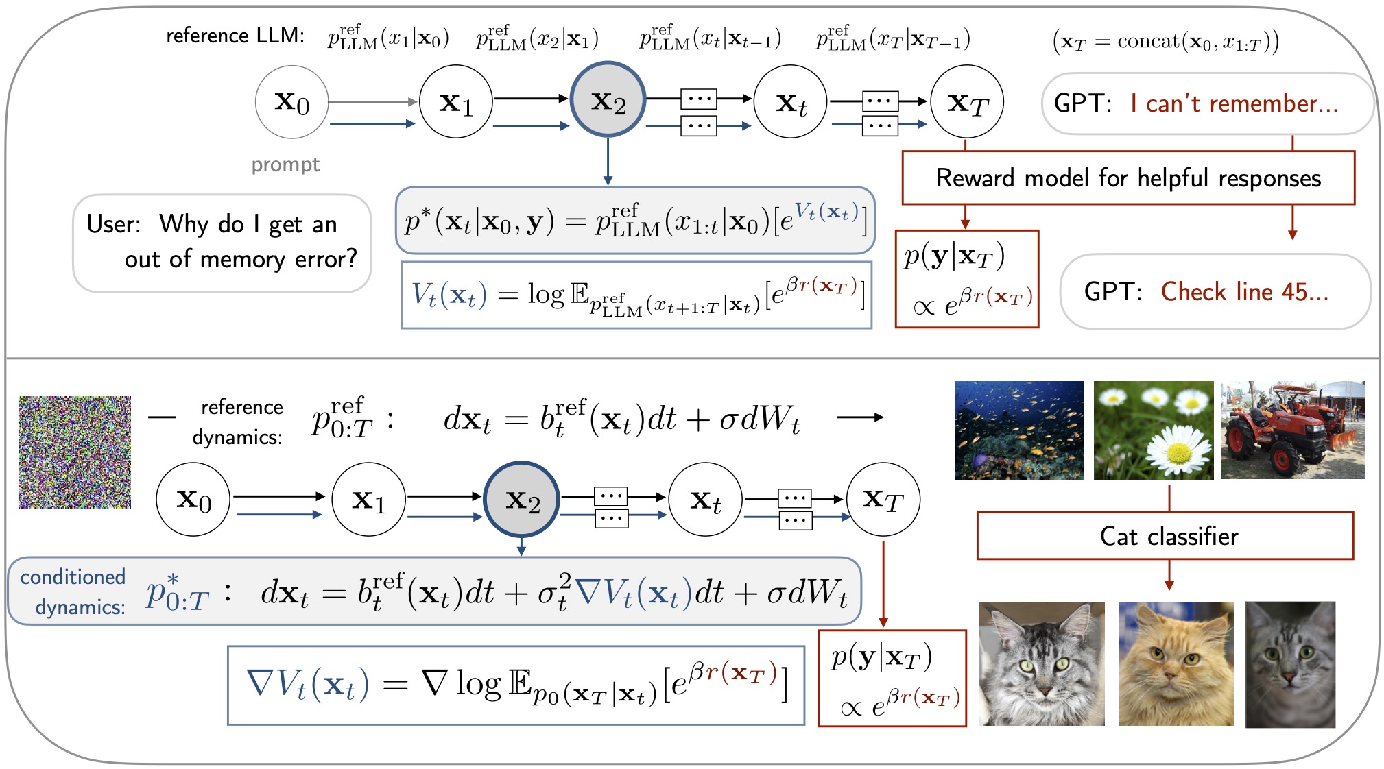
    Posterior Conditioning in both Language and Diffusion Models.  See <a href="#soft-value-function">Soft Value Function</a> and <a href="#stochastic-optimal-control">Stochastic Optimal Control</a> sections for the role of the value function.
</div>

<h2 id="target-distributions">Target Distributions</h2>
<!---For continuous models,  $$ \mathbf{x}_t \in \mathbb{R}^d $$  or in discrete models,  $$ \mathbf{x}_t \in \mathbb{R}^{d\cdot V} $$  where  $$ V $$  is the size of the vocabulary (or possible outcomes).
--->
<p>We will proceed to view many controlled generation or fine-tuning tasks as sampling from a target probability distribution at the final step  \(T\) , where the target is only known up to a normalization constant.<d-cite key="zhao2024probabilistic, uehara2024understanding, lu2024guidance, phillips2024particle"></d-cite>.   Compared to generative modeling, this task can be notably more difficult since we do not have access to samples from the target distribution.</p>

<p>To ease notation and facilitate posterior sampling interpretations,  we define an observation random variable  \(\mathbf{y}\), which is emitted as a function of the final state according to  \(p(\mathbf{y} \vert \mathbf{x}_T)\), and attempt to sample from the posterior distribution over all states,</p>

\[\begin{align}
p^*(\mathbf{x}_{0:T} \vert \mathbf{y}) = \frac{1}{\mathcal{Z}^\mathbf{y}} p^{\text{ref}}(\mathbf{x}_{0:T})p(\mathbf{y} \vert \mathbf{x}_T) \quad \qquad \mathcal{Z}^\mathbf{y} =\int p^{\text{ref}}(\mathbf{x}_{0:T})p(\mathbf{y} \vert \mathbf{x}_T) d\mathbf{x}_{0:T} \label{eq:tgt}
\end{align}\]

<p>In particular, we would like our full language model responses or final diffusion states to be distributed according to the endpoint posterior marginal \(p^*(\mathbf{x}_{T} \vert \mathbf{y})\).
We will consider a flexible class of possible target posteriors defined in the following table.</p>

<!--- While a conditioning on a particular class  $$ \mathbf{y}=c $$  or noisy observation  $$ \mathbf{y}= \mathcal{A}(\mathbf{x}_T) + \epsilon $$  are naturally written using  $$ p(\mathbf{y} \vert \mathbf{x}_T) $$ , we can accommodate a more general family of targets.   
Constraints may filter responses which factually-correct answers <d-cite key="feng2024step"></d-cite> or diffusion processes to end in a particular state or set <d-cite key="liu2023learning"></d-cite>, while reward modulation is common in both language and diffusion finetuning <d-cite key="ouyang2022training, domingo2024adjoint"></d-cite>.  .--->

<!---  In the table below, we emphasize the endpoint marginal distribution  $$ p^*(\mathbf{x}_{T} \vert \mathbf{y}) $$  associated with   $$ p^*(\mathbf{x}_{0:T} \vert \mathbf{y}) $$  above.--->

<table>
  <thead>
    <tr>
      <th>Setting</th>
      <th style="text-align: center">\(p(\mathbf{y} \vert \mathbf{x}_T)\)</th>
      <th style="text-align: center">\(p^*(\mathbf{x}_{T} \vert \mathbf{y})\)</th>
    </tr>
  </thead>
  <tbody>
    <tr>
      <td>Constraint</td>
      <td style="text-align: center">\(\mathbb{I}[\mathbf{x}_T \in \mathcal{B}]\)</td>
      <td style="text-align: center">\(\frac{1}{\mathcal{Z}^{\mathcal{B}}} p^{\text{ref}}(\mathbf{x}_{T})\mathbb{I}[\mathbf{x}_T \in \mathcal{B}]\)</td>
    </tr>
    <tr>
      <td>Classifier or Observation</td>
      <td style="text-align: center">\(p(\mathbf{y} \vert \mathbf{x}_T)\)</td>
      <td style="text-align: center">\(\frac{1}{\mathcal{Z}^\mathbf{y}} p^{\text{ref}}(\mathbf{x}_{T})p(\mathbf{y} \vert \mathbf{x}_T)\)</td>
    </tr>
    <tr>
      <td>Reward or Energy Modulation</td>
      <td style="text-align: center">\(\frac{1}{M}\exp\{ \beta~ r(\mathbf{x}_T) \}\)</td>
      <td style="text-align: center">\(\frac{1}{\mathcal{Z}^{\beta r}} p^{\text{ref}}(\mathbf{x}_{T})\exp\{ \beta~ r(\mathbf{x}_T) \}\)</td>
    </tr>
    <tr>
      <td>Arbitrary Unnormalized Density</td>
      <td style="text-align: center">\(\frac{1}{M}\frac{\tilde{\pi}_T(\mathbf{x}_T)}{p^{\text{ref}}(\mathbf{x}_T)}\)</td>
      <td style="text-align: center">\(\frac{1}{\mathcal{Z}} \tilde{\pi}_T(\mathbf{x}_T)\)</td>
    </tr>
  </tbody>
</table>

<!---In particular, we would like our full language model responses or final diffusion states to be distributed according to the endpoint posterior marginal $$ p^*(\mathbf{x}_{T} \vert \mathbf{y}) $$.
corresponds to performing rejection sampling of candidate  $$ \mathbf{x}_T $$  via the binary acceptance probability  $$ p(\mathbf{y}=1 \vert \mathbf{x}_T) = \frac{1}{M}\frac{\tilde{\pi}_T(\mathbf{x}_T)}{p^{\text{ref}}(\mathbf{x}_T)} \leq 1 $$ .
--->

<p>A crucial challenge arises from the fact that conditioning information is only provided at the terminal state  \(\mathbf{x}_T\) , whereas generation or sampling needs to be performed sequentially and forward in time according to</p>

\[\begin{align} p^*(\mathbf{x}_{0:T} \vert  \mathbf{y})= p^*(\mathbf{x}_{0} \vert \mathbf{y}) \prod_{t=1}^{T} p^*(\mathbf{x}_{t} \vert \mathbf{x}_{t-1}, \mathbf{y}) \label{eq:backward}
\end{align}\]

<p>Before describing how soft value functions and stochastic optimal control can be used to address this challenge, we discuss several concrete examples below.</p>

<h3 id="examples">Examples</h3>

<h4 id="constraints">Constraints</h4>
<p>For the language modeling setting, constraints may filter responses which correspond to correct answers to reasoning questions <d-cite key="feng2024step"></d-cite>, syntactically-valid outputs, or responses for which a scalar function meets an acceptability or rare-event threshold \(\mathbb{I}[ f(\mathbf{x}_T)\leq c]\).</p>

<p>For diffusion modeling, constraining the endpoint sample to fall within a certain set \(\mathbb{I}[ \mathbf{x}_T \in \mathcal{B}]\) corresponds to the traditional formulation of Doob’s $h$-transform, which has been used for generative modeling on constrained domains  <d-cite key="liu2023learning"></d-cite> or with aligned data <d-cite key="somnath2023aligned,du2024doob"></d-cite> arising in biomolecular or chemical problems.   In the case where \(p^{\text{ref}}\) is a diffusion with linear drift, the conditioned process ending at a particular point \(\mathbb{I}[ \mathbf{x}_T = \mathbf{x}]\)  is available as a closed form linear interpolation.   This observation underlies efficient optimization techniques for `bridge matching’ methods <d-cite key="shi2024diffusion,peluchetti2023diffusion"></d-cite> which extend rectified flow matching <d-cite key="liu2023flow,lipman2023flow"></d-cite> to stochastic processes and Schrödinger Bridge problems for generative modeling or image translation.  <d-footnote> The solution to the Schrödinger Bridge (SB) problem can be viewed as a controlled diffusion in the form of \eqref{eq:csde} and \eqref{eq:soft_value_drift}, where the control drift $u_t$ becomes a posterior expectation of the reference transition probability  <d-cite key="shi2024diffusion"></d-cite> 
$$ \begin{align*} 
u_t(\mathbf{x}_t)= \sigma_t^2 \nabla_{\mathbf{x}_t} \log p^*(\mathbf{y}|\mathbf{x}_t) &amp;= \sigma_t^2  \int d\mathbf{x}_T \frac{p^{\text{ref}}(\mathbf{x}_T|\mathbf{x}_t) p(\mathbf{y}|\mathbf{x}_T)}{\int p^{\text{ref}}(\mathbf{x}_T|\mathbf{x}_t) p(\mathbf{y}|\mathbf{x}_T) d\mathbf{x}_T} \nabla_{\mathbf{x}_t} \log p^{\text{ref}}(\mathbf{x}_T|\mathbf{x}_t)  \\
&amp;= \sigma_t^2 \mathbb{E}_{p^*(\mathbf{x}_T|\mathbf{x}_t,\mathbf{y}=1)}[ \nabla_{\mathbf{x}_t} \log p^{\text{ref}}(\mathbf{x}_T|\mathbf{x}_t)] 
\end{align*}$$   
While this fits into the General Unnormalized Target Density setting above, we do not emphasize this example since the SB problem usually assumes access to samples only. See <d-cite key="pooladian2024plug"></d-cite> for discussion, where the Sinkhorn algorithm is used to obtain a likelihood ratio ($\propto p(\mathbf{y}|\mathbf{x}_T)$) from samples and construct the control drift $ u_t $. </d-footnote></p>

<h4 id="classification-or-observation-random-variables">Classification or Observation Random Variables</h4>

<p>Given a classifier \(p(\mathbf{y}=c | \mathbf{x}_T)\), we can hope to condition our language or diffusion model to generate samples likely to be of a certain class, such as uncovering language model responses which are flagged by content moderation classifiers.   In the <a href="#stochastic-optimal-control">Stochastic Optimal Control</a> section below, we will see that class-conditioned diffusion processes characterize the optimal form of well-known guidance techniques <d-cite key="zhao2024adding"></d-cite>.
Finally, conditioning on a noisy observation \(\mathbf{y}= \mathcal{A}(\mathbf{x}_T) + \epsilon\) is natural for solving inverse problems in imaging <d-cite key="chung2022diffusion, dou2024diffusion, denker2024deft, daras2024survey"></d-cite>.</p>

<h4 id="reward-or-energy-modulation">Reward or Energy Modulation</h4>

<p>Reinforcement learning from human feedback has become a dominant paradigm for aligning pretrained language models with human preferences or task-specific applications <d-cite key="ouyang2022training"></d-cite>, finetuning diffusion models to align with text prompts or user feedback <d-cite key="domingo2024adjoint"></d-cite>, or generating proteins, molecules, or genetic sequences with particular properties such as stability, synthesizability, or downstream effectiveness .   For our purposes, we will assume a reward model is given. <br />
<!---$$ \tilde{\pi}_T(\mathbf{x}_T) =  p^{\text{ref}}(\mathbf{x}_{T})\exp\{ \beta~ r(\mathbf{x}_T) \} $$---></p>

<h4 id="general-unnormalized-target-densities">General Unnormalized Target Densities</h4>

<p>Most generally, we can seek to sample from a given target distribution over the final state \(\pi_T(\mathbf{x}_T) \propto \tilde{\pi}_T(\mathbf{x}_T)\), which is given only via its unnormalized density \(\tilde{\pi}_T(\mathbf{x}_T)\).  This includes reward modulation  \(\tilde{\pi}_T(\mathbf{x}_T) =  p^{\text{ref}}(\mathbf{x}_{T})\exp\{ \beta~ r(\mathbf{x}_T) \}\) or Boltzmann distributions as special cases.</p>

<!---Note that reward modulation is  $$ \tilde{\pi}_T(\mathbf{x}_T) =  p^{\text{ref}}(\mathbf{x}_{T})\exp\{ \beta~ r(\mathbf{x}_T) \} $$  
Note that, in these cases, we do not immediately have an observation random variable $$ p(\mathbf{y} \vert \mathbf{x}_T)$$ to  condition.--->
<p>To facilitate a posterior interpretation in these cases, we would like to introduce a random variable \(\mathbf{y}\) which reflects `optimality’, or the fact that endpoint samples are distributed according to the endpoint target.
We thus construct a hypothetical rejection sampling of the endpoint samples, where we accept samples with probability \(p(\mathbf{y}=1 \vert \mathbf{x}_T) = \frac{1}{M}\frac{\tilde{\pi}_T(\mathbf{x}_T)}{p^{\text{ref}}(\mathbf{x}_T)}\), for \(M = \max \limits_{\mathbf{x}_T}\frac{\tilde{\pi}_T(\mathbf{x}_T)}{p^{\text{ref}}(\mathbf{x}_T)}\).  The constant \(M\), which ensures \(p(\mathbf{y}=1 \vert \mathbf{x}_T) \leq 1\) and that accepted samples have the desired distribution, need not be estimated in practice, since it can be shown to vanish in the eventual posterior \(p^*(\mathbf{x}_T \vert \mathbf{y}=1)\). (see derivations here <d-footnote> In detail,  consider only the final step posterior for simplicity
$$
\begin{align*} 
p^*(\mathbf{x}_T|\mathbf{y}=1)&amp;= \frac{p^{\text{ref}}(\mathbf{x}_T)p(\mathbf{y}=1 \vert \mathbf{x}_T)}{\sum_{\mathbf{x}_T} p^{\text{ref}}(\mathbf{x}_T)p(\mathbf{y}=1 \vert \mathbf{x}_T)} \\
&amp;= \frac{p^{\text{ref}}(\mathbf{x}_T)\frac{1}{M}\frac{\tilde{\pi}_T(\mathbf{x}_T)}{p^{\text{ref}}(\mathbf{x}_T)}}{\sum_{\mathbf{x}_T} p^{\text{ref}}(\mathbf{x}_T)\frac{1}{M}\frac{\tilde{\pi}_T(\mathbf{x}_T)}{p^{\text{ref}}(\mathbf{x}_T)} } \\
&amp;= \frac{\tilde{\pi}_T(\mathbf{x}_T)}{\sum_{\mathbf{x}_T}\tilde{\pi}_T(\mathbf{x}_T) } \\
&amp;= \pi_T(\mathbf{x}_T).
\end{align*} 
$$
</d-footnote>).
<!---&=\frac{p^{\text{ref}}(\mathbf{x}_T)\frac{1}{M}\frac{\tilde{\pi}_T(\mathbf{x}_T)}{p^{\text{ref}}(\mathbf{x}_T)}}{ p^{\text{ref}}(\mathbf{x}_T)\frac{1}{M}\frac{\tilde{\pi}_T(\mathbf{x}_T)}{p^{\text{ref}}(\mathbf{x}_T)} +p^{\text{ref}}(\mathbf{x}_T)\left(1-\frac{1}{M}\frac{\tilde{\pi}_T(\mathbf{x}_T)}{p^{\text{ref}}(\mathbf{x}_T)} \right) }---></p>

<p>Again, we emphasize that this construction is hypothetical and does not affect algorithm design.  Nevertheless, it is useful to add detail to presentation in the influential 2018 tutorial by Sergey Levine <d-cite key="levine2018reinforcement"></d-cite> and facilitate our unified viewpoint in terms of posterior inference.</p>

<!---introduce a contrant $$ M = \max \limits_{\mathbf{x}_T}\frac{\tilde{\pi}_T(\mathbf{x}_T)}{p^{\text{ref}}(\mathbf{x}_T)} $$  (which need not be estimated in practice), corresponds to a rejection sampling scheme where accepting samples with probability $$ p(\mathbf{y}=1 \vert \mathbf{x}_T) = \frac{1}{M}\frac{\tilde{\pi}_T(\mathbf{x}_T)}{p^{\text{ref}}(\mathbf{x}_T)} \leq 1 $$ yields samples distributed according to $\pi_T$.
We use this construction only to provide a posterior interpretation of the target endpoint distribution, adding detail to presentation of `optimality' random variables in the influential 2018 tutorial by Sergey Levine <d-cite key="levine2018reinforcement"></d-cite>.--->

<!--- $$ p^*(\mathbf{x}_{0:T} \vert  \mathbf{y})= p^*(\mathbf{x}_{0} \vert \mathbf{y}) \prod_{t=0}^{T-1} p^*(\mathbf{x}_{t+1} \vert \mathbf{x}_{t}, \mathbf{y}) $$ 
While accepted  $$ \mathbf{x}_T $$  can then be shown to be distributed according to  $$ \pi_T(\mathbf{x}_T) $$ . However, we will see that  $$ M $$  does not need to be estimated in practice, since it is absorbed into the normalization constant  $$ \mathcal{Z} $$ . 
--->

<h3 id="initial-sampling">Initial Sampling</h3>

<p>An immediate question arises as to how to initialize sampling in \eqref{eq:backward}, since \(p^*(\mathbf{x}_{0} \vert \mathbf{y})\) is already likely to be intractable in general.</p>

<p>In language modeling settings, we are often given access to prompts $\mathbf{x}_{0}$ via data or user interaction, so it is natural to focus on the posterior over responses to particular prompts,</p>

\[\begin{align}
p^*(\mathbf{x}_{1:T} \vert \mathbf{x}_{0}, \mathbf{y}) &amp;= \frac{1}{\mathcal{Z}^{\mathbf{y}}_0(\mathbf{x}_{0})} p^{\text{ref}}(\mathbf{x}_{1:T}|\mathbf{x}_{0}) p(\mathbf{y} \vert \mathbf{x}_T) \label{eq:tgt2} \\
 \mathcal{Z}^{\mathbf{y}}_{0}(\mathbf{x}_{0}) &amp;=\int p^{\text{ref}}(\mathbf{x}_{1:T}|\mathbf{x}_{0})p(\mathbf{y} \vert \mathbf{x}_T) d\mathbf{x}_{1:T} \nonumber
\end{align}\]

<p>However, in diffusion models, we remain interested in \(p^*(\mathbf{x}_{0:T} \vert \mathbf{y})\), and risk introducing bias if our initial sampling distribution differs from $p^*(\mathbf{x}_{0} \vert \mathbf{y})$.
It may be possible to sample from \(p^*(\mathbf{x}_{0} \vert \mathbf{y}) \approx p^{\text{ref}}(\mathbf{x}_{0})\) in cases when the noising dynamics converge quickly to a stationary distribution, such as a standard Normal, regardless of the initial distribution <d-cite key="denker2024deft" section="G2"></d-cite>.  Similarly, finetuning could be performed using a `memoryless’ noise schedule which renders \(p^{\text{ref}}(\mathbf{x}_T|\mathbf{x}_{0}) = p^{\text{ref}}(\mathbf{x}_T)\) and thus \(p^*(\mathbf{x}_{0} \vert \mathbf{y})= p^{\text{ref}}(\mathbf{x}_{0})\)  <d-cite key="domingo2024adjoint"></d-cite>.   We proceed to assume \(\mathbf{x}_{0} \sim p^*(\mathbf{x}_{0} \vert \mathbf{y})\) in the diffusion setting, and focus on subsequent sampling steps for \(p^*(\mathbf{x}_{1:T} \vert \mathbf{x}_{0}, \mathbf{y})\) to encompass both language and diffusion settings.</p>

<!--- Before further discussing [Examples](#examples) for both language and diffusion models, we first proceed to introduce common mathematical tools for sequential sampling.--->

<!--- Via the sequential factorization  $$ p^*(\mathbf{x}_{1:T} \vert \mathbf{x}_{0}, \mathbf{y})=\prod_{t=0}^{T-1} p^*(\mathbf{x}_{t+1} \vert \mathbf{x}_{t}, \mathbf{y}) $$ , we will eventually be interested in sampling from the endpoint marginal  $$ p^*(\mathbf{x}_{T} \vert \mathbf{x}_{0},\mathbf{y}) $$  over full-length language responses  $$ \mathbf{x}_T =\text{concat}(\mathbf{x}_{0}, x_1, ...x_T) $$ given a prompt $$ \mathbf{x}_{0} $$  or over final diffusion states  $$ \mathbf{x}_T \in \mathbb{R}^d $$ given an initial state $$ \mathbf{x}_{0} $$.
A crucial challenge arises from the fact that conditioning information is only provided at the terminal state  $$ \mathbf{x}_T $$ , whereas generation or sampling needs to be performed sequentially and forward in time.

<!--- <d-footnote>For discrete models, note that  $$ \mathcal{Z}(\mathbf{y}) $$  integrates with respect to the counting measure on full sequences  $$ \mathbf{x}_T $$ .  The joint distribution in this expand
    <d-cite key=""></d-cite></d-footnote>
--->

<!---
 $$ \frac{1}{\mathcal{Z}(\mathcal{B})}p^{\text{ref}}(\mathbf{x}_{0:T})\mathbb{I}[\mathbf{x}_T \in \mathcal{B}] $$ 
 $$ \frac{1}{\mathcal{Z}(\mathbf{y})} p^{\text{ref}}(\mathbf{x}_{0:T})p(\mathbf{y}\\vert \mathbf{x}_T) $$ 
 $$ \frac{1}{\mathcal{Z}(\beta,r)} p^{\text{ref}}(\mathbf{x}_{0:T})\exp\{ \beta~ r(\mathbf{x}_T) \} $$   
--->
<!---
Note that reward or energy modulation can be viewed as a special case of the arbitrary target marginal with  $$ \tilde{\pi}_T(\mathbf{x}_T) =  p^{\text{ref}}(\mathbf{x}_{T})\exp\{ \beta~ r(\mathbf{x}_T) \} $$ . 
In these cases, the constant  $$ M = \max \limits_{\mathbf{x}_T}\frac{\tilde{\pi}_T(\mathbf{x}_T)}{p^{\text{ref}}(\mathbf{x}_T)} $$  corresponds to performing rejection sampling of candidate  $$ \mathbf{x}_T $$  via the binary acceptance probability  $$ p(\mathbf{y}=1 \vert \mathbf{x}_T) = \frac{1}{M}\frac{\tilde{\pi}_T(\mathbf{x}_T)}{p^{\text{ref}}(\mathbf{x}_T)} \leq 1 $$ .   Accepted  $$ \mathbf{x}_T $$  can then be shown to be distributed according to  $$ \pi_T(\mathbf{x}_T) $$ . However, we will see that  $$ M $$  does not need to be estimated in practice, since it is absorbed into the normalization constant  $$ \mathcal{Z} $$ .   This construction is simply used to provide a posterior interpretation of the target endpoint distribution, in similar fashion as the influential 2018 tutorial by Sergey Levine <d-cite key="levine2018reinforcement"></d-cite>. 

### Considering the Initial Point


| Setting      |    $$ p(\mathbf{y} \vert \mathbf{x}_T) $$      |  $$ p^*(\mathbf{x}_{T} \vert \mathbf{x}_{0} \mathbf{y}) $$   |
| ------------- |:-------------:| :-----:|
| Constraint |   $$ \mathbb{I}[\mathbf{x}_T \in \mathcal{B}] $$ |    $$ \frac{1}{\mathcal{Z}(\mathcal{B})}p^{\text{ref}}(\mathbf{x}_{T})\mathbb{I}[\mathbf{x}_T \in \mathcal{B}] $$   |
| Classifier or Observation Likelihood |   $$ p(\mathbf{y} \vert \mathbf{x}_T) $$      |  $$ \frac{1}{\mathcal{Z}(\mathbf{y})} p^{\text{ref}}(\mathbf{x}_{T})p(\mathbf{y} \vert \mathbf{x}_T) $$   |
| Reward or Energy Modulation |   $$ \frac{1}{M}\exp\{ \beta~ r(\mathbf{x}_T) \} $$     |  $$ \frac{1}{\mathcal{Z}(\beta,r)} p^{\text{ref}}(\mathbf{x}_{T})\exp\{ \beta~ r(\mathbf{x}_T) \} $$     |
| Arbitrary Target |  $$ \frac{1}{M}\frac{\tilde{\pi}_T(\mathbf{x}_T)}{p^{\text{ref}}(\mathbf{x}_T)} $$  |  $$  \frac{1}{\mathcal{Z}} \frac{p^{\text{ref}}(\mathbf{x}_{T})}{}\tilde{\pi}_T(\mathbf{x}_T) $$ |
--->

<h2 id="soft-value-function">Soft Value Function</h2>
<p>We begin by characterizing the target posterior \(p^*(\mathbf{x}_{1:T} \vert \mathbf{x}_{0}, \mathbf{y})\) via the solution to a variational optimization<d-cite key="knoblauch2022optimization"></d-cite>, which we will refer to as an Evidence Lower Bound (ELBO),
<!---\log \mathcal{Z}(\mathbb{y}) $$ ---> 
<!---
\\&=\log \int p^{\text{ref}}(\mathbf{x}_{t+1:T}\vert \mathbf{x}_{t}) p(\mathbf{y}\vert \mathbf{x}_{T}) d\mathbf{x}_{t+1:T}
$$\begin{align}
\log \mathcal{Z}(\mathbf{y}) = \max \limits_{q(\mathbf{x}_{0:T})} ~ \mathbb{E}_{q(\mathbf{x}_{0:T})}\big[ \log p(\mathbf{y}\vert \mathbf{x}_{T}) \big] - D_{KL}\big[q(\mathbf{x}_{0:T}): p^{\text{ref}}(\mathbf{x}_{0:T})\big] \label{eq:elbo}
\end{align}
 $$
---></p>

<p>\(\begin{align}
V^{\mathbf{y}}_{0}(\mathbf{x}_{0}) &amp;= \max \limits_{q(\mathbf{x}_{1:T}|\mathbf{x}_{0})} ~ \mathbb{E}_{q(\mathbf{x}_{1:T}|\mathbf{x}_{0})}\big[ \log p(\mathbf{y}\vert \mathbf{x}_{T}) \big] - D_{KL}\big[q(\mathbf{x}_{1:T}|\mathbf{x}_{0}): p^{\text{ref}}(\mathbf{x}_{1:T}|\mathbf{x}_{0})\big] \label{eq:elbo} \\
&amp;= \log \mathcal{Z}^{\mathbf{y}}_{0}(\mathbf{x}_{0})  \nonumber 
\end{align}\)
The posterior \(q(\mathbf{x}_{1:T}|\mathbf{x}_{0})= p^*(\mathbf{x}_{1:T} | \mathbf{x}_{0}, \mathbf{y}) = \frac{1}{\mathcal{Z}^{\mathbf{y}}_{0}(\mathbf{x}_{0})}  p^{\text{ref}}(\mathbf{x}_{1:T}|\mathbf{x}_{0}) p(\mathbf{y}|\mathbf{x}_T)\) achieves the maximum.<d-footnote> This can seen by solving for the the optimal $q$, subject to a normalization constraint.   Taking the variation with respect to $q$,
$$\begin{align*}
 \frac{\delta}{\delta q}[\cdot] = \log p(\mathbf{y}\vert \mathbf{x}_{T}) - \log q(\mathbf{x}_{1:T}|\mathbf{x}_{0}) + \log p^{\text{ref}}(\mathbf{x}_{1:T}|\mathbf{x}_{0}) - 1 - \lambda(\mathbf{x}_0) = 0 \\
 \implies q^*(\mathbf{x}_{1:T} | \mathbf{x}_{0}) = \frac{1}{\mathcal{Z}^{\mathbf{y}}_{0}(\mathbf{x}_{0})}p^{\text{ref}}(\mathbf{x}_{1:T}|\mathbf{x}_{0}) p(\mathbf{y}\vert \mathbf{x}_{T})
\end{align*}$$
</d-footnote>  Plugging back into \eqref{eq:elbo} and cancelling terms, we see that the soft value function corresponds to the log normalization constant  \(V^{\mathbf{y}}_{0}(\mathbf{x}_{0}) = \log \mathcal{Z}^{\mathbf{y}}_{0}(\mathbf{x}_{0})\).</p>

<!--- 
 Thus, $$ q(\mathbf{x}_{1:T}|\mathbf{x}_{0})= p^*(\mathbf{x}_{1:T} | \mathbf{x}_{0}, \mathbf{y})$$ achieves the maximum.
 Plugging back into \eqref{eq:elbo}, we see that the soft value function simplifies to the log normalization constant  $$ V^{\mathbf{y}}_{0}(\mathbf{x}_{0}) = \log \mathcal{Z}^{\mathbf{y}}_{0}(\mathbf{x}_{0}) $$ after cancellations.
 --->

<p>The optimal soft value function can be understood as translating terminal target information to intermediate steps, which facilitates sampling the exact posterior marginals along the entire trajectory.   In particular, consider the optimization \eqref{eq:elbo} starting from a given partial sequence or intermediate state \(\mathbf{x}_t\),</p>

\[\begin{align}
\hspace{-.25cm} V^{\mathbf{y}}_{t}(\mathbf{x}_t)  &amp;= \max \limits_{q(\mathbf{x}_{t+1:T}\vert \mathbf{x}_{t})} ~ \mathbb{E}_{q(\mathbf{x}_{t+1:T}\vert \mathbf{x}_{t})}\big[ \log p(\mathbf{y}\vert \mathbf{x}_{T}) \big] - D_{KL}\big[q(\mathbf{x}_{t+1:T}\vert \mathbf{x}_{t}): p^{\text{ref}}(\mathbf{x}_{t+1:T} \vert \mathbf{x}_{t})\big]  \label{eq:elbot} \\
&amp;=\log \int p^{\text{ref}}(\mathbf{x}_{t+1:T}\vert \mathbf{x}_{t}) p(\mathbf{y}\vert \mathbf{x}_{T}) d\mathbf{x}_{t+1:T}
\label{eq:int_value} \\
&amp;= \log p^*(\mathbf{y} \vert \mathbf{x}_t) \label{eq:cond_lkd}
\end{align}\]

<p>The soft value function measures the expected target likelihood under rollouts from the reference policy, which may involve generating tokens  \(x_{t+1:T}\)  or running diffusion sampling until time  \(T\).
In our setting with no intermediate reward or target information, we can recognize the expression for $V_{\mathbf{y}}^*(\mathbf{x}_t)$ in \eqref{eq:int_value} as a conditional likelihood in \eqref{eq:cond_lkd} <d-footnote>
We will find rich applications in our the setting of no intermediate reward or targets, but refer the interested reader to <d-cite key="levine2018reinforcement"></d-cite>, <d-cite key="zhao2024probabilistic" section="B"></d-cite>, <d-cite key="lu2024guidance"></d-cite> for discussion of this case in various settings.</d-footnote>
<!---
$$
\begin{align}
V^{\mathbf{y}}_{t}(\mathbf{x}_t)  = \log p^*(\mathbf{y} \vert \mathbf{x}_t)
\end{align}
$$---></p>

<h4 id="one-step-optimal-policy">One-Step Optimal Policy</h4>
<p>Similarly, we can write the one-step-ahead posterior transitions using soft values,</p>

\[\begin{align}
  p^*(\mathbf{x}_{t} \vert \mathbf{x}_{t-1}, \mathbf{y}) &amp;=  p^{\text{ref}}(\mathbf{x}_{t}|\mathbf{x}_{t-1}) \frac{p^*(\mathbf{y} \vert \mathbf{x}_t)}{p^*(\mathbf{y} \vert \mathbf{x}_{t-1})} \nonumber \\
  &amp;= p^{\text{ref}}(\mathbf{x}_{t}|\mathbf{x}_{t-1}) \exp\{ V^{\mathbf{y}}_{t}(\mathbf{x}_{t}) - V^{\mathbf{y}}_{t-1}(\mathbf{x}_{t-1}) \} \label{eq:next_token}
  \end{align}\]

<p>where \(V^{\mathbf{y}}_{t-1}(\mathbf{x}_{t-1}) = \log \mathcal{Z}^{\mathbf{y}}_{t-1} (\mathbf{x}_{t-1})\) again is the log normalization constant.</p>

<h4 id="intermediate-marginal-distributions">Intermediate Marginal Distributions</h4>
<p>Finally, composing the optimal one-step policies above, we can consider how the  target marginal distribution of \(\mathbf{x}_t\) evolves over time.  In terms of the soft value function, we have
 <!---write the evolution of the marginals in terms of the value function---></p>

<p>\(\begin{align}
p^*_{t}(\mathbf{x}_{t}\vert \mathbf{x}_{0}, \mathbf{y}) = \frac{1}{\mathcal{Z}^{\mathbf{y}}_{0}(\mathbf{x}_{0})} p^{\text{ref}}(\mathbf{x}_{t}|\mathbf{x}_{0}) \exp\{  V_\mathbf{y}^*(\mathbf{x}_{t}) \} \label{eq:marginal}
\end{align}\)
<!--which can also be seen by marginalizing backward in time  $$ p^*_{t}(\mathbf{x}_{t} \vert \mathbf{y}) = \frac{1}{\mathcal{Z}(\mathbf{y})} \int p^{\text{ref}}(\mathbf{x}_{t:T}) p(\mathbf{y} \vert \mathbf{x}_T) d\mathbf{x}_{t+1:T} $$.--->
<!---seen by marginalizing either forward  $$ p^*_{t}(\mathbf{x}_{t} \vert \mathbf{y})= \int \prod_{\tau=1}^{t-1} p^*_{\tau+1}(\mathbf{x}_{\tau+1} \vert \mathbf{x}_{\tau},\mathbf{y}) d\mathbf{x}_{0:t-1} $$ $$ = \frac{1}{\mathcal{Z}(\mathbf{y})} \int p^{\text{ref}}(\mathbf{x}_{0:t}) \exp\{  V_\mathbf{y}^*(\mathbf{x}_{t}) \} d\mathbf{x}_{0:t-1} $$  or backward in time  $$ p^*_{t}(\mathbf{x}_{t} \vert \mathbf{y}) = \frac{1}{\mathcal{Z}(\mathbf{y})} \int p^{\text{ref}}(\mathbf{x}_{t:T}) p(\mathbf{y} \vert \mathbf{x}_T) d\mathbf{x}_{t+1:T} $$ .
Finally, we will find it useful to view the value function as measuring the log importance weights between intermediate posterior and prior marginals by rearranging \eqref{eq:marginal},
---></p>

<p>where \(\mathbf{x}_0\) conditioning only affects the \(p^{\text{ref}}\) term.   We can equivalently express \eqref{eq:marginal} using likelihood ratios or logits,
\(\begin{align}
\log \frac{p^*(\mathbf{x}_{t} \vert \mathbf{x}_{0}, \mathbf{y})}{p^{\text{ref}}(\mathbf{x}_{t} | \mathbf{x}_{0})} = V^{\mathbf{y}}_{t}(\mathbf{x}_{t}) - V^{\mathbf{y}}_{0}(\mathbf{x}_{0}) = \log p^*(\mathbf{y} \vert \mathbf{x}_t) - \log \mathcal{Z}^{\mathbf{y}}_{0}(\mathbf{x}_{0})   \label{eq:logits}
\end{align}\)</p>

<p>The central message is that the optimal soft value function provides a “backward message” summarizing future conditioning information relevant to sampling at time $t$.</p>

<!---The soft value function measures the expected target likelihood under rollouts from the reference policy, which may involve generating tokens  $$ x_{t+1:T} $$  or running diffusion sampling until time  $$ T $$.  This reflects the "value" of the state $$ \mathbf{x}_t $$, and  $$ V_{\mathbf{y}}^*(\mathbf{x}_t)= \log \mathcal{Z}_t(\mathbf{x}_t;\mathbf{y}) $$  is also the normalization constant for  $$  p^*(\mathbf{x}_{t+1:T}\vert \mathbf{x}_{t},y) \propto p^{\text{ref}}(\mathbf{x}_{t+1:T}\vert \mathbf{x}_{t}) p(\mathbf{y}\vert \mathbf{x}_{T})$$ , in similar fashion to \eqref{eq:elbo}.
--->
<!---
To see how the soft value informs sequential sampling, we can recognize the one-step-ahead optimal value function  $$ V_\mathbf{y}^*(\mathbf{x}_{t+1}) $$  as an inner optimization in \eqref{eq:int_value} to write

 $$
\begin{align}
V^{\mathbf{y}}_{t}(\mathbf{x}_t)  &= \max \limits_{q(\mathbf{x}_{t+1}\vert \mathbf{x}_{t})} ~ \mathbb{E}_{q(\mathbf{x}_{t+1}\vert \mathbf{x}_{t})}\big[ V_\mathbf{y}^*(\mathbf{x}_{t+1}) \big] - D_{KL}\big[q(\mathbf{x}_{t+1} \vert \mathbf{x}_{t}): p^{\text{ref}}(\mathbf{x}_{t+1} \vert \mathbf{x}_{t})\big] \nonumber \\
& p^*_{t+1}(\mathbf{x}_{t+1} \vert \mathbf{x}_{t},\mathbf{y})  = p^{\text{ref}}(\mathbf{x}_{t+1} \vert \mathbf{x}_{t}) \exp\{  V_\mathbf{y}^*(\mathbf{x}_{t+1}) -  V_\mathbf{y}^*(\mathbf{x}_{t}) \} \label{eq:one_step}
\end{align}
 $$

where  $$ V^{\mathbf{y}}_{t}(\mathbf{x}_t)  = \log \mathcal{Z}_t(\mathbf{x}_t;\mathbf{y}) $$  again provides the normalization constant.   Finally, we use the expression for the one-step policy to write the intermediate target marginals using

 $$\begin{align}
p^*_{t}(\mathbf{x}_{t}\vert \mathbf{y}) = \frac{1}{\mathcal{Z}(\mathbf{y})} p^{\text{ref}}(\mathbf{x}_{t}) \exp\{  V_\mathbf{y}^*(\mathbf{x}_{t}) \} \label{eq:marginal}
\end{align}
 $$

which can be seen by marginalizing either forward  $$ p^*_{t}(\mathbf{x}_{t} \vert \mathbf{y})= \int \prod_{\tau=1}^{t-1} p^*_{\tau+1}(\mathbf{x}_{\tau+1} \vert \mathbf{x}_{\tau},\mathbf{y}) d\mathbf{x}_{0:t-1} $$ $$ = \frac{1}{\mathcal{Z}(\mathbf{y})} \int p^{\text{ref}}(\mathbf{x}_{0:t}) \exp\{  V_\mathbf{y}^*(\mathbf{x}_{t}) \} d\mathbf{x}_{0:t-1} $$  or backward in time  $$ p^*_{t}(\mathbf{x}_{t} \vert \mathbf{y}) = \frac{1}{\mathcal{Z}(\mathbf{y})} \int p^{\text{ref}}(\mathbf{x}_{t:T}) p(\mathbf{y} \vert \mathbf{x}_T) d\mathbf{x}_{t+1:T} $$ .
Finally, we will find it useful to view the value function as measuring the log importance weights between intermediate posterior and prior marginals by rearranging \eqref{eq:marginal},

$$\begin{align}
\log \frac{p^*(\mathbf{x}_{t} \vert  \mathbf{y})}{p^{\text{ref}}(\mathbf{x}_{t})} = V_{\mathbf{y}}^*(\mathbf{x}_{t+1}) - \log \mathcal{Z}(\mathbf{y}) \label{eq:logits}
\end{align}
$$

The central message is that the optimal soft value function provides a "backward message" summarizing future conditioning information relevant to sampling the one-step-ahead or marginal distributions at time $t$.   
--->
<h2 id="stochastic-optimal-control">Stochastic Optimal Control</h2>

<p>Remarkably, the gradient of the soft value function can also be shown to provide the optimal drift for a controlled diffusion process guiding samples to the endpoint target distribution. <br />
To build up to this connection, we note that in the continuous-time limit, the KL divergence in \eqref{eq:elbo} is finite only for path measures or SDEs of the form</p>

\[\begin{align}
Q^{u}:  \quad d\mathbf{x}_t = \left( b_t^{\text{ref}}(\mathbf{x}_t ) + u_t(\mathbf{x}_t ) \right) dt + \sigma_t dW_t, \label{eq:csde}
\end{align}\]

<p>where $u_t$ satisfies mild regularity condtiions.   In this case, the KL divergence can be written as the time-integral of the norm of \(u_t\) using the Girsanov theorem, and we can recognize the negative of the ELBO in \eqref{eq:elbo} as a stochastic optimal control problem</p>

\[\begin{align}
- V^\mathbf{y}_{0}(\mathbf{x}_{0}) = \min \limits_{Q^u(\mathbf{x}_{(0,T]}|\mathbf{x}_{0})} ~ \mathbb{E}_{Q^u(\mathbf{x}_{0:T})}\Big[ - \log p(\mathbf{y}\vert \mathbf{x}_{T}) + \int_{0}^T \frac{1}{2\sigma_t^2}\|u_t(\mathbf{x}_t)\|^2  dt  \Big] \label{eq:soc}
\end{align}\]

<p>subject to \(Q^u\) having the form of \eqref{eq:csde}.   Using variational calculus,<d-footnote> See <d-cite key="domingo2023stochastic"></d-cite> Sec. 2 and Appendix for accessible derivations. </d-footnote> one can show that the solution takes the form</p>

<p>\(\begin{align}
u_t(\mathbf{x}_t) = \sigma_t^2 \nabla_{\mathbf{x}_t} V^{\mathbf{y}}_t(\mathbf{x}_t) =  \sigma_t^2  \nabla_{\mathbf{x}_t}  \log p^*(\mathbf{y}|\mathbf{x}_t) \label{eq:soft_value_drift}
\end{align}\)
<!--- \mathbb{E}_{p^*(\mathbf{x}_T|\mathbf{x}_t, \mathbf{y})}\left[ \nabla_{\mathbf{x}_t}  \log p^{\text{ref}}(\mathbf{x}_{T}\vert \mathbf{x}_{t}) \right] 
where, in the last equality, we use take the gradient of \cref{eq:int_value} using the log-derivative identity, noting that $$ p^*(\mathbf{x}_T|\mathbf{x}_t, \mathbf{y}) = \frac{ p^{\text{ref}}(\mathbf{x}_{t+1:T}\vert \mathbf{x}_{t}) p(\mathbf{y}\vert \mathbf{x}_{T})}{ \int p^{\text{ref}}(\mathbf{x}_{t+1:T}\vert \mathbf{x}_{t}) p(\mathbf{y}\vert \mathbf{x}_{T}) d\mathbf{x}_{t+1:T}} $$ \log p^{\text{ref}}(\mathbf{x}_{t+1:T}\vert \mathbf{x}_{t}) ---></p>

<p>Using the probabilistic view of the value functions in \eqref{eq:int_value}-\eqref{eq:cond_lkd}, observe that the exponentiated value functions are related via expectations under the reference process</p>

\[\begin{align}
\exp\{ V^{\mathbf{y}}_t(\mathbf{x}_t) \} = \mathbb{E}_{p^{\text{ref}}(\mathbf{x}_{t+s} \vert\mathbf{x}_{t})}\left[ \exp\{ V^{\mathbf{y}}_{t+s}(\mathbf{x}_{t+s}) \} \right] \label{eq:value_martingale}
\end{align}\]

<p>This is known as a martingale condition in the stochastic process literature, where \(h_t^{\mathbf{y}} = \exp\{ V_t^{\mathbf{y}} \}\) is often known as Doob’s $h$-function.  The martingale condition ensures that conditional and marginals constructed from \eqref{eq:next_token}-\eqref{eq:marginal} are consistent with respect to marginalization, and results in the following remarkable theorem  <d-cite key="jamison1975markov"></d-cite>.</p>

<p><strong>Theorem 1</strong> For any function satisfying \eqref{eq:value_martingale}, the stochastic process</p>

\[\begin{align}
d\mathbf{x}_t = \left( b_t^{\text{ref}}(\mathbf{x}_t ) + \sigma^2 \nabla V_t(\mathbf{x}_t ) \right) dt + \sigma_t dW_t
\end{align}\]

<p>realizes the transition dynamics</p>

\[\begin{align}
p^V(\mathbf{x}_{t+s} | \mathbf{x}_t) = \frac{\exp\{ V_{t+s}(\mathbf{x}_{t+s})\} }{\exp\{ V_t(\mathbf{x}_t)\}} p^{\text{ref}}(\mathbf{x}_{t+s} | \mathbf{x}_t)
\end{align}\]

<p>This theorem is true for any function satisfying the martingale condition, including the optimal value function corresponding to a particular target $p^*$, and demonstrates the link between value functions, guidance drifts for controlled diffusion processes, and posterior or conditioned transition probabilities.</p>

<!--- #### Schrödinger Bridge Example
The Schrödinger Bridge or entropy-regularized optimal transport problems, which are equivalent under the choice of the Euclidean cost,<d-cite key=""></d-cite> customarily assume that samples from two target endpoint distributions are given.
The difficulty is to approximate the density ratio $$ p(\mathbf{y}|\mathbf{x}_T) \propto \frac{\tilde{\pi}(\mathbf{x}_T)}{p^{\text{ref}}(\mathbf{x}_T)} $$
to 
However, we can still use the soft value guidance perspective to interpret the optimal solution to the SB problem.  

In particular, assume we have solved the static 
--->

<h2 id="twisted-sequential-monte-carlo-sampling">Twisted Sequential Monte Carlo Sampling</h2>

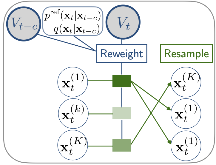
<p>In both the language and diffusion cases, we can leverage Sequential Monte Carlo to resample a set of $K$ partial sequences or intermediate states based on the (optimal) soft values, which has the effect of prioritizing sequences or states which we expect to achieve high likelihood under the final-step target distribution.</p>

<p>To introduce this importance sampling technique, we consider the unnormalized \(\tilde{p}^{*}(\mathbf{x}_{1:T} \vert \mathbf{x}_0, \mathbf{y}) = p^{\text{ref}}(\mathbf{x}_{1:T} \vert \mathbf{x}_{0}) p(\mathbf{y} \vert \mathbf{x}_T)\) (see \eqref{eq:tgt2}), which omits the intractable normalization constant \(\mathcal{Z}^\mathbf{y}_0(\mathbf{x}_0)\) and thus is easy to evaluate.  For a given proposal or approximate posterior \(q(\mathbf{x}_{1:T} \vert \mathbf{x}_0)\) (which may be learned as in <a href="#objective-functions">Objectives</a> below, or simply set to \(p^{\text{ref}}\) ), consider the importance weights in the extended space,</p>

\[\begin{align}
w_{1:T}(\mathbf{x}_{1:T}) = \frac{\tilde{p}^*(\mathbf{x}_{1:T}|\mathbf{x}_0,\mathbf{y})}{q(\mathbf{x}_{1:T}|\mathbf{x}_0)}, \qquad \mathbb{E}_{q(\mathbf{x}_{1:T}|\mathbf{x}_0)}\left[ w_{1:T}(\mathbf{x}_{1:T}) \right] = \mathcal{Z}^\mathbf{y}_0(\mathbf{x}_0) \label{eq:unbiased}
\end{align}\]

<p>The latter equality suggests that the weights are an unbiased estimator of the intractable normalization constant \(\mathcal{Z}^\mathbf{y}_0\), assuming \(w_{1:T} &lt; \infty\) for all \(\mathbf{x}_{1:T}\).</p>

<p>We would like to transform these weights into step-by-step <em>incremental</em> weights which will allow us to perform importance-weighting of intermediate states according to the optimal target posterior.  While a naive forward factorization \(w_{1:T}(\mathbf{x}_{1:T}) = p(\mathbf{y} \vert \mathbf{x}_T) \prod_{t=1}^T \frac{  p^{\text{ref}}(\mathbf{x}_{t} \vert \mathbf{x}_{t-1})}{q(\mathbf{x}_{t} \vert \mathbf{x}_{t-1})}\) would only include target information at the final step, we should instead consider the posterior transitions in \eqref{eq:backward}.   Rewriting \(p^{*}(\mathbf{x}_{t} \vert \mathbf{x}_{t-1}, \mathbf{y}) = \frac{p^*(\mathbf{y} \vert \mathbf{x}_t)}{p^*(\mathbf{y} \vert \mathbf{x}_{t-1})} p^{\text{ref}}(\mathbf{x}_{t} \vert \mathbf{x}_{t-1})\) using \eqref{eq:next_token}, we have</p>

\[\begin{align}
w_{1:T}(\mathbf{x}_{1:T}) &amp;= \prod_{t=1}^T \frac{p^*(\mathbf{x}_{t} \vert \mathbf{x}_{t-1}, \mathbf{y})}{q(\mathbf{x}_{t} \vert \mathbf{x}_{t-1})} \nonumber \\
&amp;= \prod_{t=1}^T \frac{p^*(\mathbf{y} \vert \mathbf{x}_t)}{p^*(\mathbf{y} \vert \mathbf{x}_{t-1})} \frac{p^{\text{ref}}(\mathbf{x}_{t} \vert \mathbf{x}_{t-1})}{q(\mathbf{x}_{t} \vert \mathbf{x}_{t-1})} =  \prod_{t=1}^T \frac{\exp\{ V^{\mathbf{y}}_{t}(\mathbf{x}_{t}) \}}{\exp\{ V^{\mathbf{y}}_{t-1}(\mathbf{x}_{t-1}) \}} \frac{p^{\text{ref}}(\mathbf{x}_{t} \vert \mathbf{x}_{t-1})}{q(\mathbf{x}_{t} \vert \mathbf{x}_{t-1})} \label{eq:weights}
\end{align}\]

<!---which has an equivalent expression using value functions $$ p^*(\mathbf{y} \vert \mathbf{x}_t)=\exp\{ V^{\mathbf{y}}_{t}(\mathbf{x}_{t}) \} $$, see \eqref{eq:next_token}. --->
<p>Note,the numerator at the final step includes the given target conditional \(p(\mathbf{y} \vert \mathbf{x}_T)\).</p>

<div style="width: 40%;  margin: auto; text-align: center;">
        <figure>

  <picture>
    

    <!-- Fallback to the original file -->
    <img src="/assets/img/2025-01-06-soft-value-guidance/smc_small.png" class="img-fluid rounded z-depth-1" width="auto" height="auto" onerror="this.onerror=null; $('.responsive-img-srcset').remove();" />

  </picture>

</figure>

</div>
<!----  
<div style="width: 40%; margin: auto; text-align: center;">
    <img src="/assets/img/2025-01-06-soft-value-guidance/smc_small.png" class="img-fluid rounded z-depth-1" alt="SMC diagram">
</div>
--->

<p>The weights in \eqref{eq:weights} suggest a sequential resampling scheme at intermediate steps.   For a budget of \(K\) samples and looping over timesteps \(1 \leq t \leq T\), we can proceed with the following steps:</p>
<ul>
  <li>for \(t \in [1, T]\):
    <ul>
      <li>for \(k \in [1, K]\):
        <ul>
          <li>Sample \(\mathbf{x}_t^{(k)} \sim q(\mathbf{x}_t \vert \mathbf{x}_{t-1}^{(k)})\)</li>
          <li>Update weights \(w_{1:t}^{(k)} = w_{1:t-1}^{(k)} \frac{p^*(\mathbf{y} \vert \mathbf{x}_t^{(k)})}{p^*(\mathbf{y} \vert \mathbf{x}_{t-1}^{(k)})} \frac{p^{\text{ref}}(\mathbf{x}_{t}^{(k)} \vert \mathbf{x}_{t-1}^{(k)})}{q(\mathbf{x}_{t}^{(k)} \vert \mathbf{x}_{t-1}^{(k)})}\)</li>
        </ul>
      </li>
      <li>(if resampling condition met, perform multinomial resampling):
        <ul>
          <li>Sample \(i_k \sim \text{categorical}\left( \Big\{ \frac{w_{1:t}^{(j)}}{\sum_{j=1}^K w_{1:t}^{(\ell)}} \Big\}_{j=1}^K   \right)\) for \(k \in [1,K]\)</li>
          <li>Copy or Reassign Samples: \(\mathbf{x}_t^{(k)} \gets \mathbf{x}_t^{(i_k)}\) ( for all \(k \in [1,K]\) in parallel)</li>
          <li>Reset weights:  \(w_{1:t}^{(k)} \gets  \frac{1}{K} \sum_{j=1}^K w_{1:t}^{(j)}\)</li>
        </ul>
      </li>
    </ul>
  </li>
</ul>

<p>Note that resetting the weights means that only subsequent weights are used for resampling at future timesteps, which preserves the unbiasedness of the eventual weights in \eqref{eq:unbiased}.  See the blog post by Tuan Anh Le for an elegant proof <d-cite key="tuan2023unbiased"></d-cite>.  More advanced resampling techniques such as systematic resampling might also be used.</p>

<p>Finally, we can use this resampling scheme even for approximate \(V^{\theta}_{t}(\mathbf{x}_{t})\) or \(p^\theta(\mathbf{y} \vert \mathbf{x}_{t})\) for \(t &lt; T\), although it is clear that the efficacy of this scheme will depend on the quality of these intermediate value functions or likelihoods.</p>

<!---So long as we use the exact target information at the endpoint $$ p(\mathbf{y} \vert \mathbf{x}_T) $$, one can show that the weights are unbiased in the sense of \eqref{eq:unbiased}.  A blog post by Tuan Anh Le provides a particularly simple proof <d-cite key="tuan2023unbiased"></d-cite>.--->

<h4 id="language">Language</h4>
<p>For the language modeling setting, recall that we absorbed the autoregressive model into Markov transitions \(p^{\text{ref}}(\mathbf{x}_{t} \vert \mathbf{x}_{t-1})=p^{\text{ref}}_{\text{LM}}(x_{t} \vert \mathbf{x}_{t-1}) \mathbb{I}[\mathbf{x}_{t} =\text{concat}(\mathbf{x}_{t-1}, x_{t})]\) where the states expand with concatenation of next tokens.
Rewriting the proposal in similar terms, we can think of the weights as evolving according to</p>

\[\begin{align}
w_{1:T}(\mathbf{x}_{1:T}) &amp;= \prod_{t=1}^T \frac{p(\mathbf{y} \vert \mathbf{x}_t)}{p(\mathbf{y} \vert \mathbf{x}_{t-1})} \frac{p^{\text{ref}}_{\text{LM}}(x_t \vert \mathbf{x}_{t-1})}{q_{\text{LM}}(x_t \vert \mathbf{x}_{t-1})} =  \prod_{t=1}^T \frac{\exp\{ V^{\mathbf{y}}_{t}(\mathbf{x}_{t}) \}}{\exp\{ V^{\mathbf{y}}_{t-1}(\mathbf{x}_{t-1}) \}} \frac{p^{\text{ref}}_{\text{LM}}(x_t \vert \mathbf{x}_{t-1})}{q_{\text{LM}}(x_t \vert \mathbf{x}_{t-1})} \nonumber 
\end{align}\]

<p>where the likelihood or values are evaluated on the partial sequences \(\mathbf{x}_t\) and \(\mathbf{x}_{t-1}\).   See <d-cite key="tuan2022twoviews"></d-cite> or <d-cite key="zhao2024probabilistic"></d-cite> for additional discussion.</p>

<h4 id="diffusion">Diffusion</h4>
<p>Since diffusion process operate on states \(\mathbf{x}_{t} \in \mathbb{R}^d\) in Markovian fashion, the weights in \eqref{eq:weights} can be used as is, where \(q(\mathbf{x}_{t} \vert \mathbf{x}_{t-1})\) corresponds to the discretization of a stochastic process as in \eqref{eq:csde}.</p>

<!---
As we saw in \eqref{eq:marginal}, the optimal value functions $$V^t_{\mathbf{y}} = \log p(\mathbf{y}|\mathbf{x}_t) $$ parameterize the intermediate marginals of the endpoint target distribution.    


While the optimal values are not available in practice, we note that approximate values can be also be used (see [Objectives](#objective-functions) below). <d-footnote> As long as the final step is reweighted according to the true unnormalized target distribution, then the resulting sampling and estimation will be exact in the limit as $$ K \rightarrow \infty $$. </d-footnote>


based on the soft values $$V^t_{\mathbf{y}} = \log p(\mathbf{y}|\mathbf{x}_t)  $$  which 
has the effect of prioritizing partial sequences or intermediate states with high target likelihood in expectation over the terminal $$\mathbf{x}_T$$.

according to their importance weights 


under a sequence of marginal distributions.  

We will discuss learning or approximating the value function in [Objectives](#objective-functions), but first discuss how (approximate) value functions can be used to sample intermediate target marginals.   


For well-learned value functions, has the effect of prioritizing partial sequences or intermediate states with high target likelihood $$  \log p(\mathbf{y}|\mathbf{x}_t) $$, in expectation over the terminal $$\mathbf{x}_T$$.

--->

<h2 id="objective-functions">Objective Functions</h2>
<p>We finally discuss several classes of objective functions for learning value functions and/or approximate posterior policies.  We only attempt to give a high-level landscape of various methods, mostly in discrete time, and defer to references for algorithmic and technical details.</p>

<h3 id="evidence-lower-bound-mode-seeking-kl">Evidence Lower Bound (Mode-Seeking KL)</h3>
<p>Similarly to derivations in the case of standard variational inference, one can show that, for a given \(q\), the gap in the ELBO in \eqref{eq:elbo} is the mode-seeking KL divergence \(D_{KL}\big[ q(\mathbf{x}_{1:T} | \mathbf{x}_{0}) : p^*(\mathbf{x}_{1:T} | \mathbf{x}_{0}, \mathbf{y})\big]\).   Thus, minimizing this KL divergence corresponds to maximizing \eqref{eq:elbo}. Notably, since \(q(\mathbf{x}_{1:T} | \mathbf{x}_{0})\) appears in the first argument, optimizing this objective requires taking gradients through the sampling procedure.</p>

<h4 id="language-1">Language</h4>
<p>When \(\log p(\mathbf{y}\vert \mathbf{x}_{T}) = \beta ~ r(\mathbf{x}_{T}) - \log M\) , we recognize \eqref{eq:elbo} as a common objective for reinforcement learning from human feedback in language models, where \(q(\mathbf{x}_{1:T}|\mathbf{x}_0)\) is optimized using policy gradient methods such as PPO <d-cite key="ouyang2022training"></d-cite> or REINFORCE <d-cite key="ahmadian2024back"></d-cite>. While PPO maintains a value network to reweight policy gradients, the focus is on finetuning a policy \(q^{\phi}(\mathbf{x}_{1:T}|\mathbf{x}_0)\), and an optimal policy \(q = p^*\) will implicitly capture the value functions through the next-token logits in \eqref{eq:next_token}.  A similar observation underlies token-wise interpretations of direct preference optimization parameterizations <d-cite key="rafailov2024r"></d-cite>.   Nevertheless, learned value functions may also be used to guide generative sampling, either through Monte Carlo Tree Search <d-cite key="liu2023making"></d-cite> or Sequential Monte Carlo  <d-cite key="zhao2024probabilistic"></d-cite>(as above).</p>

<h4 id="diffusion-1">Diffusion</h4>

<p>Methods for solving stochastic control problems have an extensive history dating back to <d-cite key="pontryagin1962mathematical"></d-cite>.  Directly solving \eqref{eq:soc} using backpropagation through trajectories is known as the adjoint method  <d-cite key="li2020scalable, kidger2021efficient"></d-cite>, for which improved gradient estimators have been recently proposed in <d-cite key="domingo2024adjoint"></d-cite>.  The adjoint method was used for sampling from general unnormalized target densities in <d-cite key="zhang2022path"></d-cite>.</p>

<h3 id="cross-entropy-mass-covering-kl">Cross Entropy (Mass-Covering KL)</h3>

<p>While the ELBO and mode-seeking KL divergence was used to introduce the target distribution as the solution of a variational optimization in \eqref{eq:elbo}, we can perform optimization using any divergence minimization technique with the desired optimum.   One example is to optimize the mass-covering KL divergence as in maximum likelihood training of energy-based models, where recognizing the form of the optimal target marginals in \eqref{eq:marginal}, we optimize</p>

\[\begin{align} 
\min \limits_{\theta} \sum_{t=1}^T D_{KL}\big[ p^*(\mathbf{x}_{1:t} \vert \mathbf{x}_{0}, \mathbf{y}) :  p^{\text{ref}}(\mathbf{x}_{1:t} \vert \mathbf{x}_{0}) \exp\{V^\theta_t(\mathbf{x}_t) \}/\mathcal{Z}_{V^\theta}(\mathbf{x}_0) \big] 
\end{align}\]

<p>Although exact samples from \(p^*(\mathbf{x}_{1:t} \vert \mathbf{x}_{0}, \mathbf{y})\) are usually not available, one may use importance sampling approximations to reweight samples according to the endpoint target information \(p(\mathbf{y} \vert \mathbf{x}_T )\), and reuse these weights for approximate sampling at intermediate \(t\). <d-cite key="lu2023contrastive, zhao2024probabilistic"></d-cite></p>

<h4 id="language-2">Language</h4>

<p>For full-sequence policy optimization with the only loss at the final-step \(T\), the distributional policy gradient algorithm  <d-cite key="khalifa2020distributional, go2023aligning"></d-cite> amounts to optimizing the mass-covering KL, where the energy is parameterized directly via a normalized policy \(q^{\phi}(\mathbf{x}_{1:T} \vert \mathbf{x}_0)\).   For learning intermediate value functions, contrastive twist learning <d-cite key="zhao2024probabilistic"></d-cite> optimizes a marginal KL divergence at each step, learning the value functions \(V^{\mathbf{y}}_{t}\) as energies.</p>

<h4 id="diffusion-2">Diffusion</h4>

<p>The contrastive energy prediction objective in <d-cite key="lu2023contrastive"></d-cite> amounts to approximate energy-based training of the value functions \(V^{\mathbf{y}}_{t}\) at each step, which can then be used to guide sampling using \(\nabla V^{\mathbf{y}}_{t}\)  as a guidance or control drift in \eqref{eq:csde}.</p>

<p>For sampling from a general target density, <d-cite key="phillips2024particle"></d-cite> learn intermediate value functions for guidance and SMC resampling using a `target score matching’ loss <d-cite key="de2024target"></d-cite>. This loss requires importance sampling corrections to draw approximate samples from the endpoint target distribution \(p^{*}(\mathbf{x}_T \vert \mathbf{y})\) (as in the mass-covering KL), but the loss directly regresses against the gradient of the target energy or log unnormalized density.</p>

<h3 id="path-consistency">Path Consistency</h3>

<p>Path Consistency objectives <d-cite key="nachum2017bridging"></d-cite> consider enforcing the first-order optimality conditions associated with the optimization in \eqref{eq:elbo}-\eqref{eq:elbot} using a squared error loss.   Since this is a functional equality which should hold everywhere, we can optimize the loss over some off-policy sampling distribution \(\pi_s(\mathbf{x}_{1:T}\vert\mathbf{x}_0)\).    Taking the variation of \eqref{eq:elbo}-\eqref{eq:elbot} with respect to \(q\) yields a KKT condition, which we can enforce using</p>

\[\begin{align}
\min \limits_{\theta,\phi} \mathbb{E}_{\pi_s(\mathbf{x}_{1:T}\vert\mathbf{x}_0)}\left[\left(   \log p(\mathbf{y}\vert \mathbf{x}_{T})  - V^{\theta}_{0}(\mathbf{x}_0)  -  \log \frac{q^\phi(\mathbf{x}_{1:T}\vert \mathbf{x}_{0})}{p^{\text{ref}}(\mathbf{x}_{1:T} \vert \mathbf{x}_{0})} \right)^2 \right]
\end{align}\]

<p>This may also be viewed as minimizing the square of the log importance weights between full-sequence forward and reverse processes in \eqref{eq:unbiased}-\eqref{eq:weights}.<d-cite key="zhao2024probabilistic" section="App C1"></d-cite>
Note that we may also construct one- or $c$-step consistency losses for any \(1 \leq t \leq t + c \leq T\) using the compositional structure of the optimal values in \eqref{eq:elbot}-\eqref{eq:marginal} or decomposition of weights in \eqref{eq:weights},</p>

\[\begin{align}
\min \limits_{\theta,\phi} \mathbb{E}_{\pi_s(\mathbf{x}_{1:T}\vert\mathbf{x}_0)}\left[\left(   V^{\theta}_{t+c}(\mathbf{x}_{t+c}) - V^{\theta}_{t}(\mathbf{x}_t)  -  \sum_{\tau=t+1}^{t+c} \log \frac{q^\phi(\mathbf{x}_{\tau} \vert \mathbf{x}_{\tau-1})}{p^{\text{ref}}(\mathbf{x}_{\tau} \vert \mathbf{x}_{\tau-1})} \right)^2 \right]
\end{align}\]

<p>Non-zero intermediate rewards would also appear in the loss.</p>

<h4 id="language-3">Language</h4>

<p>Path consistency losses correspond to (partial) `trajectory balance’ losses in the literature on Generative Flow networks (GFlowNets), and have been applied for inference <d-cite key="hu2023amortizing"></d-cite> and finetuning <d-cite key="guo2022efficient"></d-cite> in autoregressive language models.</p>

<h4 id="diffusion-3">Diffusion</h4>
<p>Trajectory balance or path consistency losses can also be applied for inference in diffusions models <d-cite key="venkatraman2024amortizing"></d-cite>, see also <d-cite key="uehara2024understanding" ref-section="Sec 6"></d-cite>.  In the sampling literature, a similar principle underlies the <em>log-variance</em> divergences studied in <d-cite key="nusken2021solving, richter2023improved"></d-cite>, in which we enforce that the log likelihood ratio of <em>path-measures</em> or stochastic processes be constant or equal to zero.   Recent work <d-cite key="chen2024sequential"></d-cite> has also married these losses with intermediate SMC resampling.</p>

<h3 id="denoising-mean-approximation-for-diffusion-settings">Denoising Mean Approximation for Diffusion Settings</h3>

<p>Diffusion models parameterized via denoising mean prediction \(\hat{\mathbf{x}}_T = D_\theta(t,\mathbf{x}_t)\) provide a particularly convenient, <em>training-free</em> estimator of intermediate value functions.   Instead of fully estimating the expectation in \eqref{eq:int_value} or \eqref{eq:value_martingale}, one can make a single-sample approximation by evaluating \(p(\mathbf{y}\vert \hat{\mathbf{x}}_T)\) at the denoising mean prediction,</p>

\[\begin{align}
V^{\mathbf{y}}_t(\mathbf{x}_t)  = \log \mathbb{E}_{p^{\text{ref}}(\mathbf{x}_{T} \vert\mathbf{x}_{t})}\left[ p(\mathbf{y}\vert\mathbf{x}_T) \right]  \approx \log p(\mathbf{y}\vert\hat{\mathbf{x}}_T)
\end{align}\]

<p>From this approximation, we can construct an approximate guidance drift \(\nabla \hat{V}^{\mathbf{y}}_t(\mathbf{x}_t) \approx \nabla \log p(\mathbf{y}\vert\hat{\mathbf{x}}_T)\) (for differentiable likelihoods) along with targets \(\hat{V}^{\mathbf{y}}_t(\mathbf{x}_t)\) for intermediate SMC resampling in \eqref{eq:weights}  <d-cite key="wu2024practical"></d-cite>.
This approximation has found wide applicability for inverse problems <d-cite key="chung2022diffusion"></d-cite>, protein generation <d-cite key="wu2024practical"></d-cite>, and images <d-cite key="anonymous2024alignment"></d-cite> for continuous diffusion models, along with recent applications for discrete diffusion models <d-cite key="li2024derivative"></d-cite>.   However, given that this estimator can be crude even in simple cases <d-cite key="phillips2024particle"></d-cite>, 
recent work <d-cite key="anonymous2024alignment"></d-cite> finds benefits to annealing the contribution of these terms for both guidance and SMC.</p>

<h2 id="conclusion">Conclusion</h2>

<p>In this blog post, we have proposed to understand controlled generation, sampling, and guidance in both language and diffusion models through the lens of probabilistic inference.   Through connections with soft reinforcement learning and stochastic optimal control, we obtain a rich design space of objective functions for learning both approximate posterior distributions and value functions, which can also be used within sequential importance sampling techniques to improve generation and estimation.   We hope that this overview provides useful conceptual tools for newcomers to these rapidly-evolving areas, while also contributing to the continued cross-pollination of ideas (i) between language and diffusion model literatures, (ii) between particular problem settings within the diffusion literature, or (iii) between sampling, RL, and finetuning literatures.<d-footnote>Thanks to Yuanqi Du for feedback on a draft of this post.</d-footnote></p>

<!--- The full Schrödinger Bridge (SB) problem is solved by a controlled stochastic differential equation in \eqref{eq:csde} with the value function as the drift, which amounts to taking a posterior expectation of the gradient of the reference likelihood $$ \nabla V^t_{\mathbf{y}}(\mathbf{x}_t) = \mathbb{E}_{p^*( \mathbf{x}_T \vert \mathbf{x}_t)}\left[ \nabla \log p^{\text{ref}}(x_T \vert x_t) \right]$$, which can be seen by differentiating \eqref{eq:value_grad}.   Since the SB problem assumes samples are given, the Sinkhorn algorithm can be used to solve for the potentials or likelihood ratios and used in a plug-in estimator of the vector field  (see <d-cite key="pooladian2024plugin"></d-cite> for discussion). --->]]></content><author><name>Rob Brekelmans</name></author><summary type="html"><![CDATA[]]></summary></entry></feed>